Machine learning for malware detection

Plop,

I have been reading many articles about Machine Learning recently, and it seems to be the new hype technology so I wanted to play a bit with these algorithms to better understand the principles behind it. If you don’t know machine learning, you should to read this awesome article or this one. This article was largely inspired by this one which analyze the Titanic data.

Machine Learning and Classification#

So the idea of machine learning is to let the algorithm learn by itself the best parameters from data in order to make good predictions. There are many different applications, in our case we will consider using machine learning algorithm to classify binaries between legitimate and malicious binaries. This idea is not new and Adobe has even released a tool called Adobe Malware Classifier at Black Hat 2012 but it will be a nice exercice to see how to use machine learning.

Here is the plan that we will follow :

• Extract as many features as we can from binaries to have a good training data set. The features have to be integers or floats to be usable by the algorithms
• Identify the best features for the algorithm : we should select the information that best allows to differenciate legitimate files from malware.
• Choose a classification algorithm
• Test the efficiency of the algorithm and identify the False Positive/False negative rate

Feature Extraction from binaries#

As I said earlier, machine learning only uses integer or float data as features for detection, but it is not a big deal as most PE parameters are integers (field size, addresses, parameters…). So I extracted all the PE parameters I could by using pefile, and considered especially the one that are relevant for identifying malware, like the entropy of section for packer detection. As we can only have a fix list of feature (and not one per section), I extracted the Mean, Minimum and Maximum of entropy for sections and resources.

Here is the final list of feature extracted : Name, md5, Machine, SizeOfOptionalHeader, Characteristics, MajorLinkerVersion, MinorLinkerVersion, SizeOfCode, SizeOfInitializedData, SizeOfUninitializedData, AddressOfEntryPoint, BaseOfCode, BaseOfData, ImageBase, SectionAlignment, FileAlignment, MajorOperatingSystemVersion, MinorOperatingSystemVersion, MajorImageVersion, MinorImageVersion, MajorSubsystemVersion, MinorSubsystemVersion, SizeOfImage, SizeOfHeaders, CheckSum, Subsystem, DllCharacteristics, SizeOfStackReserve, SizeOfStackCommit, SizeOfHeapReserve, SizeOfHeapCommit, LoaderFlags, NumberOfRvaAndSizes, SectionsNb, SectionsMeanEntropy, SectionsMinEntropy, SectionsMaxEntropy, SectionsMeanRawsize, SectionsMinRawsize, SectionMaxRawsize, SectionsMeanVirtualsize, SectionsMinVirtualsize, SectionMaxVirtualsize, ImportsNbDLL, ImportsNb, ImportsNbOrdinal, ExportNb, ResourcesNb, ResourcesMeanEntropy, ResourcesMinEntropy, ResourcesMaxEntropy, ResourcesMeanSize, ResourcesMinSize, ResourcesMaxSize, LoadConfigurationSize, VersionInformationSize.

Many other feature could have been considered, for instance the number of suspicious function imported, or the number of section with a abnormal name, but it will be for another time (I ended the script a bit late in the night and forgot to implement those ¯\(ツ)/¯ ).

Regarding the dataset, we need to have an important number of both legitimate and malicious file:

• For legitimate file, I gathered all the Windows binaries (exe + dll) from Windows 2008, Windows XP and Windows 7 32 and 64 bits, so exactly 41323 binaries. It is not a perfect dataset as there is only Microsoft binaries and not binaries from application which could have different properties, but I did not find any easy way to gather easily a lot of legitimate binaries, so it will be enough for playing
• Regarding malware, I used a part of Virus Share collection by downloading one archive (the 134th) and kept only PE files (96724 different files).

I used pefile to extract all these features from the binaries and store them in a csv file (ugly code is here, data are here).

And here we are with a large CSV file (138048 lines) ready for playing!

Feature Selection#

The idea of feature selection is to reduce the 54 features extracted to a smaller set of feature which are the most relevant for differentiating legitimate binaries from malware.

To play with the data, we will use Pandas and then Scikit which largely uses the numpy library:

data = pd.read_csv('data.csv', sep='|')
legit_binaries = data[0:41323].drop(['legitimate'], axis=1)
malicious_binaries = data[41323::].drop(['legitimate'], axis=1)

So a first way of doing it manually could be to check the different values and see if there is a difference between the two groups. For instance, we can take the parameter FileAlignment (which defines the alignment of sections and is by default 0x200 bytes) and check the values :

In [8]: legit_binaries['FileAlignment'].value_counts()
Out[8]:
512      36843
4096      4313
128         89
32          40
65536       36
16           2
Name: FileAlignment, dtype: int64

In [9]: malicious_binaries['FileAlignment'].value_counts()
Out[9]:
512     94612
4096     2074
128        18
1024       15
64          2
32          1
16          1
2048        1
Name: FileAlignment, dtype: int64

So if we remove the 20 malware having weird values here, there is not much difference on this value between the two groups, this parameter would not make a good feature for us.

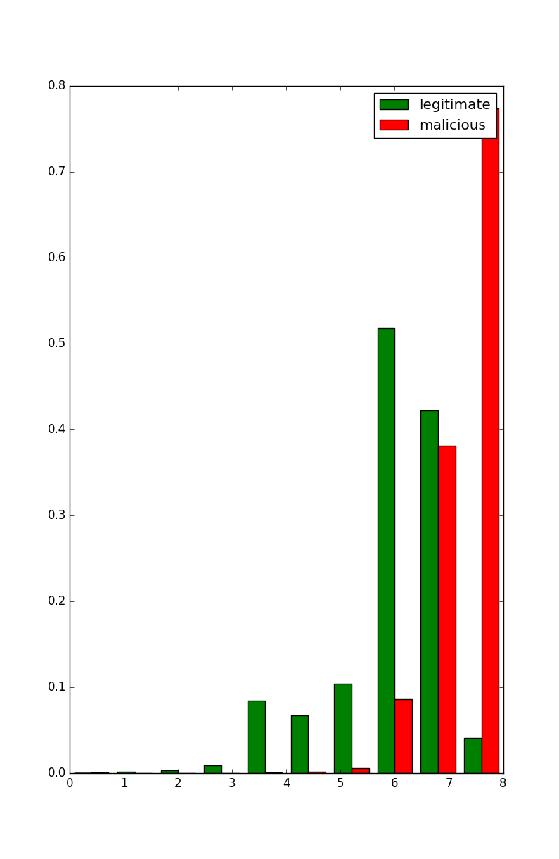
On the other side, some values are clearly interesting like the max entropy of the sections which can be represented with an histogram:

In [12]: plt.hist([legit_binaries['SectionsMaxEntropy'], malicious_binaries['SectionsMaxEntropy']], range=[0,8], normed=True, color=["green", "red"],label=["legitimate", "malicious"])
Out[12]:
([array([ 0.        ,  0.00120095,  0.00129333,  0.00914567,  0.08896238,
        0.04665213,  0.12609933,  0.55631513,  0.37580371,  0.04452738]),
  array([  9.04607814e-05,   0.00000000e+00,   1.29229688e-05,
           1.55075625e-04,   5.16918751e-04,   1.51198735e-03,
           6.04794938e-03,   8.64675840e-02,   3.81266348e-01,
                                            7.73930754e-01])],
  array([ 0. ,  0.8,  1.6,  2.4,  3.2,  4. ,  4.8,  5.6,  6.4,  7.2,  8. ]),
  <a list of 2 Lists of Patches objects>)

In [13]: plt.legend()
Out[13]: <matplotlib.legend.Legend at 0x7f15da65ee10>

In [14]: plt.show()

But there is a more efficient way of selecting features : some algorithms have been developed to identify the most interesting features and reduce the dimensionality of the data set (see the Scikit page for Feature Selection).

In our case, we will use the Tree-based feature selection:

In [15]: X = data.drop(['Name', 'md5', 'legitimate'], axis=1).values

In [16]: y = data['legitimate'].values

In [17]: fsel = ske.ExtraTreesClassifier().fit(X, y)

In [20]: model = SelectFromModel(fsel, prefit=True)

In [21]: X_new = model.transform(X)

In [22]: X.shape
Out[22]: (110258, 54)

In [23]: X_new.shape
Out[23]: (110258, 11)

So in this case, the algorithm selected 11 important features among the 54, and we can notice that indeed the SectionsMaxEntropy is selected but other features (like the Machine value) are surprisingly also good parameters for this classification :

In [1]: nb_features = X_new.shape[1]

In [2]: indices = np.argsort(fsel.feature_importances_)[::-1][:nb_features]

In [3]: for f in range(nb_features):
   ...:         print("%d. feature %s (%f)" % (f + 1, data.columns[2+indices[f]], fsel.feature_importances_[indices[f]]))
      ...:
      1. feature Characteristics (0.187685)
      2. feature Machine (0.173019)
      3. feature ImageBase (0.099215)
      4. feature Subsystem (0.091090)
      5. feature MajorSubsystemVersion (0.077067)
      6. feature SectionsMaxEntropy (0.046552)
      7. feature SizeOfOptionalHeader (0.040004)
      8. feature ResourcesMaxEntropy (0.035633)
      9. feature VersionInformationSize (0.027091)
      10. feature SectionsNb (0.020562)
      11. feature DllCharacteristics (0.018640)

Selection of the Classification Algorithm#

The best classification algorithm depends on many parameters and some of them (like SVM) have a lot of different parameters and can be difficult to correctly configure. So I used a simple option: I tested some of them with default parameters and selected the best one (I removed SVM because it does not handle well dataset with many features):

algorithms = {
        "DecisionTree": tree.DecisionTreeClassifier(max_depth=10),
        "RandomForest": ske.RandomForestClassifier(n_estimators=50),
        "GradientBoosting": ske.GradientBoostingClassifier(n_estimators=50),
        "AdaBoost": ske.AdaBoostClassifier(n_estimators=100),
        "GNB": GaussianNB()
    }

results = {}
print("\nNow testing algorithms")
for algo in algorithms:
    clf = algorithms[algo]
    clf.fit(X_train, y_train)
    score = clf.score(X_test, y_test)
    print("%s : %f %%" % (algo, score*100))
    results[algo] = score

winner = max(results, key=results.get)
print('\nWinner algorithm is %s with a %f %% success' % (winner, results[winner]*100))

Let’s run it:

Now testing algorithms
GNB : 69.478450 %
DecisionTree : 98.960522 %
RandomForest : 99.351684 %
AdaBoost : 98.558493 %
GradientBoosting : 98.761318 %

Winner algorithm is RandomForest with a 99.351684 % success

If we recompute the false positive/false negative rate on the test data, we obtain :

• False positive : 0.568241 %
• False negative : 0.830565 %

So it’s a 99.35% success, so more than the Adobe work (98.21%) but still with the RandomForest algorithm.

The whole code for feature selection and algorithm test is available here

Reuse the algorithm#

So now we want to reuse this algorithms for detection, we can just save the object and the feature list :

joblib.dump(algorithms[winner], 'classifier/classifier.pkl')
open('classifier/features.pkl', 'w').write(pickle.dumps(features))

I have then implemented a simple tool which load the feature list and the classifier, extract the PE feature and predict if a binary is malicious or not:

> python2 checkpe.py ~/virusshare/VirusShare_000b296200f7b8fffbc584f3eac864b2
The file VirusShare_000b296200f7b8fffbc584f3eac864b2 is malicious
> python2 checkpe.py ~/legitimate/explorer.exe
The file explorer.exe is legitimate

As I like the new Manalyzer platform, I have also developed a script which download the PE properties and predict if the binary is legitimate of not:

>python2 checkmanalyzer.py https://manalyzer.org/report/a9ea61c5ae7eab02c63955336a7c7efe
The file a9ea61c5ae7eab02c63955336a7c7efe is legitimate
> python2 checkmanalyzer.py https://manalyzer.org/report/9c5c27494c28ed0b14853b346b113145
The file 9c5c27494c28ed0b14853b346b113145 is malicious

Why it’s not enough?#

First, a bit of vocabulary for measuring IDS accuracy (taken from Wikipedia):

• Sensitivity : the proportion of positives identified as such (or true positive rate)
• Specificity : the proportion of negatives correctly identified as such (or true negative)
• False Positive Rate (FPR) : the proportion of events badly identified as positive over the total number of negatives
• False Negative Rate (FNR) : the proportion of events badly identified as negative over the total number of positives

So why 99.35% is not enough?

Because you can’t just consider the sensitivity/specificity of the algorithm, you have to consider the malicious over legitimate traffic ratio to understand how many alerts will be generated by the IDS. And this ratio is extremely low.

Let’s consider the you have 1 malicious event every 10 000 event (it’s a really high ratio) and 1 000 000 events per day, you will have :

• 100 malicious events, 99 identified by the tool and 1 false negative (0.83% FNR but let’s consider 1% here)
• 999 900 legitimate events, around 6499 identified as malicious (0.65% FPR)

So in the end, the analyst would received 6598 alerts per day with only 99 true positive in it (1.5%). Your IDS is useless here. (Out of curiosity, the same problem applies when detecting cancer at large scale (in French))

If we take our example, a standard Windows 7 install has around 15000 binary files (it seems to be very different depending on the version, but let’s say 15000), which means that in average 97 files would be detected incorrectly as malicious. And that’s a bad antivirus.

Conclusion#

So it was a fun example of machine learning utilization. I like how Pandas and Scikit make machine learning easy to use in python (and Scikit is really well explained and documented!). I was really surprised to have such good results without any effort for configuring the algorithm specifically for this context, and it shows that the Adobe tool is not as good as I thought.

Still, it is interesting to remind the IDS problem and show it concretely (just after self-congratulation for such a good sensitivity :).

If you have any question, comment or idea to continue playing with this dataset, let me know on Twitter.

Here are some nice references on this topic:

• Learning Pandas in 10 minutes
• Would You Survive the Titanic? A Guide to Machine Learning in Python
• Scikit Learn

Adéu!

Edit 21/07/16: improved the dataset with more legitimate binaries. Updated the results Edit 02/08/16: explained why it’s not enough

This article was written mainly while listening Glenn Gould Goldberg Variations (1955)